 CS660 Combinatorial Algorithms
Fall Semester, 1996
Dynamic Programming
[To Lecture Notes Index]
San Diego State University -- This page last updated Nov 5, 1996

Contents of Dynamic Programming
- References
- Optimal BST
- Dynamic Programming
Mehlhorn's Text, pages 177-187
Introduction to Algorithms, Chapter 16
Assume:
- We have a list of n items: a1, a2, ...,
an
- Key(ak) = ak
- Probability of accessing item ak is known in advance and is
P(ak)
- The list is ordered by keys, a1 <= a2 <= ...
an
How to produce the BST that has the least search cost given the access
probability for each key?
Optimal BST
Greedy Algorithm fails
Example:
-
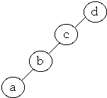
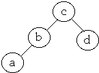
- list = a, b, c, d
- P(a) = .1, P(b) = .2, P(c) = .3, P(d) = .4
-
-
-

-
-
- Average Cost = 1*0.4 + 2*0.3 + 3*0.2 + 4*0.1 = 2.0
- Optimal BST

- Average Cost = 1*0.3 + 2*0.4 + 2*0.2 + 3*0.1 = 1.8
Finding the Optimal BST
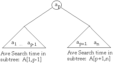
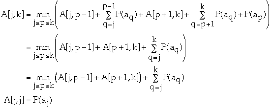
Let A[j, k] = minimum average search time for a binary search tree with items
aj <= aj+1 <= ... ak
How to find A[1,n]?Set p = 1, 2, ..., n


| j\k | 0 | 1 | 2 | 3 | 4 | 5 |
| 1 | 0 | P(a1) | A[1,2] | | | |
| 2 | 0 | 0 | P(a2) | | A[2,4] | |
| 3 | 0 | 0 | 0 | P(a3) | | |
| 4 | 0 | 0 | 0 | 0 | P(a4) | |
| 5 | 0 | 0 | 0 | 0 | 0 | P(a5) |
| 6 | 0 | 0 | 0 | 0 | 0 | 0 |
Time Complexity for finding Optimal BST [[Theta]](n3)
"Dynamic programming algorithm stores the results for small subproblems and
looks them up, rather than recomputing them, when it needs them later to solve
larger subproblems"
Baase
"Dynamic programming algorithm is very useful approach to many optimization
problems. ... Usually, we can find a tailor-made algorithm which is more
efficient than the straight-forward algorithm based on dynamic programming"
T. C. Hu
Steps in developing a dynamic programming algorithm
Characterize the structure of an optimal solution
Recursively define the value of an optimal solution
Compute the value of an optimal solution in a bottom-up fashion
Construct an optimal solution from computed information
Matrix-chain Multiplication
The Problem
Let A be a 10 * 100 matrix,
-
- B be a 100 * 5 matrix
- C be a 5 * 50 matrix
- Then
- A * B is a 10 * 5 matrix
- B * C is a 100 * 50 matrix
Computing
-
- A * B takes 10 * 100 * 5 = 5,000 multiplications
-
- (A * B) * C takes 10 * 5 * 50 = 2,500 additional mult.
-
- So (A * B) * C requires total of 7,500 multiplications
Computing
-
- B * C takes 100 * 5 * 50 = 25,000 multiplications
-
- A * (B * C) takes 10 * 100 * 50 = 50,000 additional mult.
-
- So A * (B * C) requires total of 75,000 multiplications
But (A * B) * C = A * (B * C)
Matrix-chain Multiplication
The Problem
Given a chain <A1, A2, ..., An>
matrices, where matrix Ak has dimension pk-1 *
pk fully parenthesize the product A1* A2*...
*An, in a way that minimizes the number of scalar
multiplications
Characterize the structure of an optimal solution
Optimal solution is of the form:
- (A1* ... *Ak) * (Ak+1* ... *An)
not showing the parentheses in (A1* ... *Ak) or in
(Ak+1* ... *An)
We must use the optimal parenthesization of A1* ... *Ak
and the optimal parenthesization of Ak+1* ... *An
Thus the optimal solution to an instance of the matrix-chain multiplication
problem contains within it optimal solutions to subproblem instances
That is it is recursive
Recursively define the value of an optimal solution
Recall matrix Ak has dimension pk-1 * pk for
k = 1,..., n
Let m[k, w] be the minimum the number of scalar multiplications needed to
compute Ak* ... *Aw
If (Ak* ... *Az) * (Az+1* ... *Aw)
is the optimal solution then
- m[k, w] = m[k, z] + m[z+1, w] + pk-1 * pz *
pk
since (Ak* ... *Az) is a pk-1 * pz
matrix
and (Az+1* ... *Aw) is a pz * pw
matrix
But what is z?

Compute the optimal solution in a bottom-up fashion

Example
| Matrix | dimension | r | pr |
| A1 | 10*20 | 0 | 10 |
| A2 | 20*3 | 1 | 20 |
| A3 | 3*5 | 2 | 3 |
| A4 | 5*30 | 3 | 5 |
| | 4 | 30 |
| 1 | 2 | 3 | 4 |
| 1 | 0 | 600 | 750 | 1950 |
| 2 | | 0 | 300 | 2250 |
| 3 | | | 0 | 450 |
| 4 | | | | 0 |


Construct an optimal solution
from computed information
Example
| Matrix | dimension | r | pr |
| A1 | 10*20 | 0 | 10 |
| A2 | 20*3 | 1 | 20 |
| A3 | 3*5 | 2 | 3 |
| A4 | 5*30 | 3 | 5 |
| | 4 | 30 |
| 1 | 2 | 3 | 4 |
| 1 | A1 | A1A2 | (A1A2)A3 | (A1A2)(A3A4) |
| 2 | | A2 | A2A3 | A2(A3A4) |
| 3 | | | A3 | A3A4 |
| 4 | | | | A4 |


Time Complexity of building the OBST?
We have a list of n items: a1, a2, ..., an
Probability of accessing item ak is P(ak)
Let A[j, k] = minimum average search time for a binary search tree with items
aj <= aj+1 <= ... ak

Let root[j,k] = p that gave the minimum value for A[j, k]
That is root[j,k] = root of OBST for items aj, a2, ...,
ak
Let w[j,k] = P(aj) + P(aj+1) + ... +
P(ak)
Constructing the OBST
for k = 1 to n do
- A[k, k] = P(ak)
- A[k, k-1] = 0
- root[k,k] = k
- w[k, k] = P(ak)
end
A[n+1, n] = 0
for diagonal = 1 to n -1 do
- for j = 1 to n - diagonal do
- k = j + diagonal
-
- w[j, k] = w[j, k - 1] + P(ak)
-
- let p, j <= p <= k, be the value minimizes:
-

-
- root[j,k] = p
-
- A[j, k] = A[j, p-1] + A[p+1, k] + w[j, k]
- end for
end for
Example 1
| k | 1 | 2 | 3 | 4 | 5 | 6 |
| ak | a | b | c | d | e | f |
| P(ak)'s = | 0.4 | 0.05 | 0.15 | 0.05 | 0.1 | 0.25 |
root
| 1 | 1 | 1 | 1 | 1 | 3 |
| 0 | 2 | 3 | 3 | 3 | 5 |
| 0 | 0 | 3 | 3 | 3 | 5 |
| 0 | 0 | 0 | 4 | 5 | 6 |
| 0 | 0 | 0 | 0 | 5 | 6 |
| 0 | 0 | 0 | 0 | 0 | 6 |
A
| 0 | 0.4 | 0.5 | 0.85 | 1 | 1.35 | 2.1 |
| 0 | 0 | 0.05 | 0.25 | 0.35 | 0.6 | 1.2 |
| 0 | 0 | 0 | 0.15 | 0.25 | 0.5 | 1.05 |
| 0 | 0 | 0 | 0 | 0.05 | 0.2 | 0.6 |
| 0 | 0 | 0 | 0 | 0 | 0.1 | 0.45 |
| 0 | 0 | 0 | 0 | 0 | 0 | 0.25 |
| 0 | 0 | 0 | 0 | 0 | 0 | 0 |

Example 2
P(ak)'s = (0.15 0.025 .05 .025 .05 .125 .025 .075 0.075 .05 .15 .075
.05 .025 .05)
Root
| 1 | 1 | 1 | 1 | 1 | 3 | 3 | 6 | 6 | 6 | 6 | 6 | 6 | 6 | 6 |
| 0 | 2 | 3 | 3 | 3 | 5 | 6 | 6 | 6 | 6 | 6 | 9 | 9 | 9 | 11 |
| 0 | 0 | 3 | 3 | 3 | 5 | 6 | 6 | 6 | 6 | 9 | 9 | 9 | 9 | 11 |
| 0 | 0 | 0 | 4 | 5 | 6 | 6 | 6 | 6 | 6 | 9 | 9 | 9 | 9 | 11 |
| 0 | 0 | 0 | 0 | 5 | 6 | 6 | 6 | 6 | 8 | 9 | 9 | 9 | 11 | 11 |
| 0 | 0 | 0 | 0 | 0 | 6 | 6 | 6 | 8 | 8 | 9 | 9 | 11 | 11 | 11 |
| 0 | 0 | 0 | 0 | 0 | 0 | 7 | 8 | 8 | 9 | 9 | 11 | 11 | 11 | 11 |
| 0 | 0 | 0 | 0 | 0 | 0 | 0 | 8 | 8 | 9 | 9 | 11 | 11 | 11 | 11 |
| 0 | 0 | 0 | 0 | 0 | 0 | 0 | 0 | 9 | 9 | 11 | 11 | 11 | 11 | 11 |
| 0 | 0 | 0 | 0 | 0 | 0 | 0 | 0 | 0 | 10 | 11 | 11 | 11 | 11 | 11 |
| 0 | 0 | 0 | 0 | 0 | 0 | 0 | 0 | 0 | 0 | 11 | 11 | 11 | 11 | 11 |
| 0 | 0 | 0 | 0 | 0 | 0 | 0 | 0 | 0 | 0 | 0 | 12 | 12 | 12 | 13 |
| 0 | 0 | 0 | 0 | 0 | 0 | 0 | 0 | 0 | 0 | 0 | 0 | 13 | 13 | 13 |
| 0 | 0 | 0 | 0 | 0 | 0 | 0 | 0 | 0 | 0 | 0 | 0 | 0 | 14 | 15 |
| 0 | 0 | 0 | 0 | 0 | 0 | 0 | 0 | 0 | 0 | 0 | 0 | 0 | 0 | 15 |
A[1,15] = 2.925
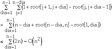
Modified Algorithm
for diagonal = 1 to n -1 do
- for j = 1 to n - diagonal do
- k = j + diagonal
- w[j, k] = w[j, k - 1] + P(ak)
-
- let p, root[j,k-1] <= p <= root[j+1,k], be the value
minimizes:

-
- root[j,k] = p
-
- A[j, k] = A[j, p-1] + A[p+1, k] + w[j, k]
- end for
end for
Time Complexity

General Theorem
Let H(i, j) be a real number for 1 <= i < j <= n
Let c(i, j) be defined by:
- c(i, i) = 0
-
- c(i, j) = H(i, j) +

Let K(i, j) = largest k, i <= k <=j, that minimizes c(i, k-1) + c(k,
j)
H(i, j) is monotone with respect to set inclusion of intervals if
- H(j, k) <= H(x, y) if j <= x < y <= k
H(i, j) satisfies the quadrangle inequality (QI) if
- H(j, k) + H(x, y) <= H(x, k) + H(j, y) if j <= x < k <=
y
Theorem. If H(i, j) satisfies QI and is monotone then c(i, j) can be
computed in time O(n2)
Lemma. If H(i, j) satisfies QI and is monotone then c(i, j) satisfies
QI
Lemma. If c(i, j) satisfies QI then we have
-
- K(i, j) <= K(i, j+ 1) <= K(i+1, j+1)
 CS660 Combinatorial Algorithms
 CS660 Combinatorial Algorithms