CS 660: Optimal BST

CS 660: Combinatorial Algorithms
Optimal BST

[To Lecture Notes Index]
San Diego State University -- This page last updated November 13, 1995

Contents of Optimal BST Lecture

References

Mehlhorn's Text, pages 177-187

Introaduction to Algorithms, Chapter16

Optimal BST

Assume:

We have a list of n items: a1, a2, ..., an

Key(ak) = ak

Probability of accessing item ak is known in advance and is P(ak)

The list is ordered by keys, a1 <= a2 <= ... an

How to produce the BST that has the least search cost given the access probability for each key?

Optimal BST Greedy Algorithm fails
Example:


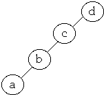
list = a, b, c, d

P(a) = .1, P(b) = .2, P(c) = .3, P(d) = .4





Average Cost = 1*0.4 + 2*0.3 + 3*0.2 + 4*0.1 = 2.0

Optimal BST

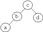
Average Cost = 1*0.3 + 2*0.4 + 2*0.2 + 3*0.1 = 1.8

Finding the Optimal BST
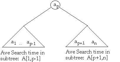
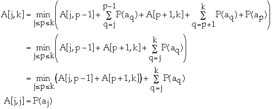
Let A[j, k] = minimum average search time for a binary search tree with items aj <= aj+1 <= ... ak
How to find A[1,n]?Set p = 1, 2, ..., n

j\k	1	2	3	4	5
1	P(a1)
2	0	P(a2)		A[2,4]
3	0	0	P(a3)
4	0	0	0	P(a4)
5	0	0	0	0	P(a5)
6	0	0	0	0	0

Time Complexity for finding Optimal BST Theta(n³)

"Dynamic programming algorithm stores the results for small subproblems and looks them up, rather than recomputing them, when it needs them later to solve larger subproblems"

Baase

"Dynamic programming algorithm is very useful approach to many optimization problems. ... Usually, we can find a tailor-made algorithm which is more efficient than the straight-forward algorithm based on dynamic programming"

T. C. Hu

Steps in developing a dynamic programming algorithm

Characterize the structure of an optimal solution

Recursively define the value of an optimal solution

Compute the value of an optimal solution in a bottom-up fashion

Construct an optimal solution from computed information

Matrix-chain Multiplication The Problem
Let A be a 10 * 100 matrix,


B be a 100 * 5 matrix
C be a 5 * 50 matrix

Then

A * B is a 10 * 5 matrix
B * C is a 100 * 50 matrix

Computing


A * B takes 10 * 100 * 5 = 5,000 multiplications

(A * B) * C takes 10 * 5 * 50 = 2,500 additional mult.

So (A * B) * C requires total of 7,500 multiplications

Computing


B * C takes 100 * 5 * 50 = 25,000 multiplications

A * (B * C) takes 10 * 100 * 50 = 50,000 additional mult.

So A * (B * C) requires total of 75,000 multiplications

But (A * B) * C = A * (B * C)

Matrix-chain Multiplication The Problem
Given a chain <A1, A2, ..., An> matrices, where matrix Ak has dimension pk-1 * pk fully parenthesize the product A1* A2*... *An, in a way that minimizes the number of scalar multiplications

Characterize the structure of an optimal solution

Optimal solution is of the form:

(A1* ... *Ak) * (Ak+1* ... *An)

not showing the parentheses in (A1* ... *Ak) or in (Ak+1* ... *An)

We must use the optimal parenthesization of A1* ... *Ak and the optimal parenthesization of Ak+1* ... *An

Thus the optimal solution to an instance of the matrix-chain multiplication problem contains within it optimal solutions to subproblem instances

That is it is recursive

Recursively define the value of an optimal solution
Recall matrix Ak has dimension pk-1 * pk for k = 1,..., n

Let m[k, w] be the minimum the number of scalar multiplications needed to compute Ak* ... *Aw

If (Ak* ... *Az) * (Az+1* ... *Aw) is the optimal solution then

m[k, w] = m[k, z] + m[z+1, w] + pk-1 * pz * pk

since (Ak* ... *Az) is a pk-1 * pz matrix

and (Az+1* ... *Aw) is a pz * pw matrix

But what is z?

Compute the optimal solution in a bottom-up fashion

Example

Matrix		dimension		r		pr
A1		10*20			0		10	
A2		20*3			1		20
A3		3*5			2		3
A4		5*30			3		5
					4		30

	1	2	3	4
1	0	600	750	1950
2		0	300	2250
3			0	450
4				0

Construct an optimal solution from computed information
Example

Matrix		dimension		r		pr
A1		10*20			0		10	
A2		20*3			1		20
A3		3*5			2		3
A4		5*30			3		5
					4		30

	1	2	3	4
1	A1	A1A2	(A1A2)A3	(A1A2)(A3A4)
2		A2	A2A3	A2(A3A4)
3			A3	A3A4
4				A4

Time Complexity of building the OBST?
We have a list of n items: a1, a2, ..., an

Probability of accessing item ak is P(ak)

Let A[j, k] = minimum average search time for a binary search tree with items aj <= aj+1 <= ... ak

Let root[j,k] = p that gave the minimum value for A[j, k]

That is root[j,k] = root of OBST for items aj, a2, ..., ak

Let w[j,k] = P(aj) + P(aj+1) + ... + P(ak)

Constructing the OBST
for k = 1 to n do

A[k, k] = P(ak)
A[k, k-1] = 0
root[k,k] = k
w[k, k] = P(ak)

end
A[n+1, n] = 0

for diagonal = 1 to n -1 do

for j = 1 to n - diagonal do
k = j + diagonal w[j, k] = w[j, k - 1] + P(ak) let p, j <= p <= k, be the value minimizes: root[j,k] = p A[j, k] = A[j, p-1] + A[p+1, k] + w[j, k]
end for

end for

Example 1

k	1	2	3	4	5	6
ak	a	b	c	d	e	f
P(ak)'s =   0.4	0.05	0.15	0.05	0.1	0.25

root

1	1	1	1	1	3
0	2	3	3	3	5
0	0	3	3	3	5
0	0	0	4	5	6
0	0	0	0	5	6
0	0	0	0	0	6

0	0.4	0.5	0.85	1	1.35	2.1
0	0	0.05	0.25	0.35	0.6	1.2
0	0	0	0.15	0.25	0.5	1.05
0	0	0	0	0.05	0.2	0.6
0	0	0	0	0	0.1	0.45
0	0	0	0	0	0	0.25
0	0	0	0	0	0	0

Example 2
P(ak)'s = (0.15 0.025 .05 .025 .05 .125 .025 .075 0.075 .05 .15 .075 .05 .025 .05)

Root

1	1	1	1	1	3	3	6	6	6	6	6	6	6	6
0	2	3	3	3	5	6	6	6	6	6	9	9	9	11
0	0	3	3	3	5	6	6	6	6	9	9	9	9	11
0	0	0	4	5	6	6	6	6	6	9	9	9	9	11
0	0	0	0	5	6	6	6	6	8	9	9	9	11	11
0	0	0	0	0	6	6	6	8	8	9	9	11	11	11
0	0	0	0	0	0	7	8	8	9	9	11	11	11	11
0	0	0	0	0	0	0	8	8	9	9	11	11	11	11
0	0	0	0	0	0	0	0	9	9	11	11	11	11	11
0	0	0	0	0	0	0	0	0	10	11	11	11	11	11
0	0	0	0	0	0	0	0	0	0	11	11	11	11	11
0	0	0	0	0	0	0	0	0	0	0	12	12	12	13
0	0	0	0	0	0	0	0	0	0	0	0	13	13	13
0	0	0	0	0	0	0	0	0	0	0	0	0	14	15
0	0	0	0	0	0	0	0	0	0	0	0	0	0	15

A[1,15] = 2.925

Modified Algorithm
for diagonal = 1 to n -1 do

for j = 1 to n - diagonal do
k = j + diagonal
w[j, k] = w[j, k - 1] + P(ak)

let p, root[j,k-1] <= p <= root[j+1,k], be the value minimizes:

root[j,k] = p

A[j, k] = A[j, p-1] + A[p+1, k] + w[j, k]
end for

end for

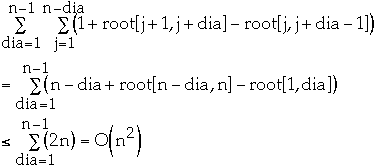
Time Complexity

General Theorem
Let H(i, j) be a real number for 1 <= i < j <= n

Let c(i, j) be defined by:

c(i, i) = 0

c(i, j) = H(i, j) +

Let K(i, j) = largest k, i <= k <=j, that minimizes c(i, k-1) + c(k, j)

H(i, j) is monotone with respect to set inclusion of intervals if

H(j, k) <= H(x, y) if j <= x < y <= k

H(i, j) satisfies the quadrangle inequality (QI) if

H(j, k) + H(x, y) <= H(x, k) + H(j, y) if j <= x < k <= y

Theorem. If H(i, j) satisfies QI and is monotone then c(i, j) can be computed in time O(n²)

Lemma. If H(i, j) satisfies QI and is monotone then c(i, j) satisfies QI

Lemma. If c(i, j) satisfies QI then we have

: K(i, j) <= K(i, j+ 1) <= K(i+1, j+1)

Splay vs. OBST

Recall in OBST we have:

We have a list of n items: a1, a2, ..., an and leaves b0, b1, ..., bn

Probability of accessing item ak is P(ak) = Alphak

Let Betak be the probability of accessing a key that is between ak and ak+1, that is leaf bk

In splay tree we have Betak = 0, and Alphak = q(i)/m

Theorem 9: Let Popt be the be the weighted path length of optimum BST. We have:


where H = H(Beta0 ,Alpha1 ,Beta1 , Alpha2, Beta2,... , Alphan, Betan) is entropy

Thus we have:

for some x

Since Popt is the average path length the total time spent to perform m accesses is m*Popt.
Now:

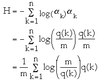
So m*H =

Thus: m*Popt <= m*H + 1 =

+ m

Nearly Optimal BST

We have a list of n items: a1, a2, ..., an

Probability of accessing item ak is P(ak)

k 1 2 3 4 5 6
ak a b c d e f
P(ak)'s = 0.4 0.05 0.15 0.05 0.1 0.25
Method 1

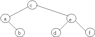
Average Access Cost = 2.2 Nearly Optimal BST k 1 2 3 4 5 6
ak a b c d e f
P(ak)'s = 0.4 0.05 0.15 0.05 0.1 0.25 Method 2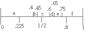

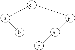
Average Access Cost = 2.1

Optimal Alphabetic Tree [1]

An alphabetic tree is a binary search tree in which all data is in the leaves. Internal nodes are used in search for the data

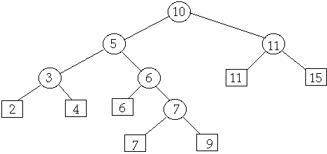
Let V1, V2,... Vn be the order of the leaves

Let wk be the weight, or frequency of access, of leaf Vk

Combining Vk and Vp, denote their parent node by Vkp and it weight wkp = wk+ wp

All leaves are square nodes, all parents are round nodes
Optimal Alphabetic Tree: Definitions

Two nodes are a compatible pair if they are adjacent or if all nodes between them are round nodes

The weight of a pair is the weight of the parent of the two nodes

A pair with minimum weight over all pairs is a minimum pair

Minimum compatible pair is the compatible pair with the least weight over all compatible pairs

Ties are broken by taking the pair with the left most left node

If two compatible pairs have the same left node and the same weight, then pick the pair with the leftmost right node

Hu-Tucker Algorithm
1. Construction

Find the minimum compatible pair
Replace the left node of the pair by the pair's parent
Remove right node of the pair

Repeat n-1 times

Call the resultant tree T'

2. Level Assignment

Determine the level number Lk of every leaf Vk in T'

3. Reconstruction

We have the level numbers L1, L2,... Ln of all leaves

Find the leftmost maximum level number, say Lk = q

Then Lk+1 = q

Replace Lk and Lk+1 with a parent node with level q - 1

Repeat n - 1 times

Theorem. The Hu-Tucker algorithm can be implemented to produce the optimal alphabetic tree with N leaves in O(Nlg(N)) time and O(N) space How Well Does OBST and NOBST Perform?
We have a list of n items: a1, a2, ..., an and leaves b0, b1, ..., bn

Probability of accessing item ak is known in advance and is P(ak) = Alphak

Let Betak be the probability of accessing a key that is between ak and ak+1, that is leaf bk

The list is ordered by keys, b0< a1 <b1< a2 < ... < an < bn

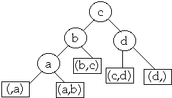
(Beta0 ,Alpha1 ,Beta1 , Alpha2, Beta2,... , Alphan, Betan) is the access distribution

Let

Let L(ak) be the level of the node ak

Let

P is the weighted path length of a tree

Let (Gamma1 ,Gamma2,... , Gamman) be a discrete probability distribution, i.e.

Gammak >= 0 and SigmaGammak =1

H(Gamma1 ,Gamma2,... , Gamman) =

is the entropy of the distribution. ( 0*log 0 = 0)

Let TBB be the tree resulting from the nearly optimal BST algorithm 1

Theorem 7[2]: Let L(ak) be the depth of node ak and let L(bk) be the depth of leaf bk in tree TBB Then


bk <= floor (log 1/bk) + 2
ak <= floor (log 1/ak)

Theorem 8[3]: Let PBB be the weighted path length of the tree TBB. Then

Theorem 9[4]: Let PBB be the weighted path length of tree TBB. Let Popt be the be the weighted path length of optimum BST. We have:


where H = H(Beta0 ,Alpha1 ,Beta1 , Alpha2, Beta2,... , Alphan, Betan) and

This gives us

Example.
In English, the probability of occurrence of the i-th most frequent word is approximately[5]

This yields

H(Alpha1 ,Alpha2, ... ) = 10.2

The weighted path length of an optimum binary search tree for all English words is no larger than 11.2. Nearly Optimal BST
We have a list of n items: a1, a2, ..., an

Probability of accessing item ak is P(ak)

k 1 2 3 4 5 6
ak a b c d e f
P(ak)'s = 0.4 0.05 0.15 0.05 0.1 0.25
Method 1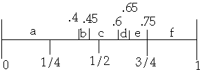

Problem:

k 1 2 3
ak a b c
P(ak)'s = 0.45 0.1 0.45

Algorithm for Nearly Optimal Lexicographic Tree [6]

Given the ordered set {a} of names, such that a1 <= a2 <= ... an , and two parameters, F and N0

(1) If N <= N0 , use dynamic programming.

(2) If N> N0, let W[k, l] be the weight of the subtree with frequencies

Betak ,Alphak+1 ,Betak+1 , ... , Alphal, Betal

F a parameter and AC the centroid.
Form the ordered set of names {AF} = {AL} union AC,
where the members of the set {AL} satisfy

|W[O,L-1] - W[L,N]| < W[O,N]/F, 1 <= F <= W[O,N]

(3) Find an index, max, such that Alphamax = maximum Alphai, where ai is in {AF}.
(4) If in the set {AF} there is at least one name preceding or equal to AC with associated frequency Alphamax, let p be the index such that ap with Alphap = Alphamax, is lexicographically closest to AC.

If there is no such p, let {AQ} be the null set and go to Step 6.

(5) If ap is the first member of {AF} and Alphap-1 > Alphap, form the set {AQ} = {ap-1 , ap-2, ., au}, where Alphap-j-1 > Alphap-j , j = 0, ... ,p-u-1 and Alphau-1 <= Alphau or u-p = floor(lg N);

if ap is not the first member of {AF}, let {AQ} be the null set.

(6) If in the set {AF} there is at least one name following or equal to AC with associated frequency Alphamax let r be the index such that ar with Alphar = Alphamax is lexicographically closest to AC;

if there is no such r, let {AS} be the null set and go to Step 8.

(7) If ar is the last member of {AF} and Alphar<Alphar+1, form the set {AS}= {ar+1, ar+2,...,av}, where Alphar+j<Alphar+j+1, j=0, 1, ... ,v-r-1, and Alphav>=Alphav+1or v-r = floor(lg N).

If ar is not the last member of {AF}, let {AS} be the null set.

(8) Find an index, root, such that Alpharoot = maximum Alphai, where ai is in {AQ} union {AF}union{AS} and |W[O,root-1] - W[root,N]| is minimized; choose aroot as the root of the tree.

(9) Go to Step 1 and repeat the algorithm for the subtrees a1, a2, ... aroot-1 and aroot+1, ... aN, where N is root-I and N-root for the two cases.

Picking N0 and F
if Beta/Alpha is small (<= 3) than use N0= 15

if Beta/Alpha is large (> 3) than use N0= 25 or 30

if Beta/Alpha is large (> 2) than use F = 6

if Beta/Alpha ~ 1 than use F = 4

if Beta/Alpha < 1 than use F = 4

The tree takes O(Nlog(N)) to construct

Average search time for NOBST is within 2% of the average search time of the OBST Average Search Length
N0= 15, F = 5

N	Alpha freq	Beta freq	OBST	NOBST
5	19,846	982,497	3.4114	3.4114
15	42,653	959,690	4.2864	4.2864
25	60,087	942,256	5.0638	5.1033
50	92,117	910,226	6.0483	6.1461
100	138,975	863,368	7.0007	7.0437
150	173,157	829,186	7.4885	7.5503
200	200,412	801,931		7.8795
500	305,266	697,077		8.9606
1000	401,288	601,055		9.6490
3000	561,956	440,387		10.6220
6000	655,538	346,805		11.1177
12000	740,022	262,321		11.1592

CS 660: Combinatorial Algorithms Optimal BST