 CS 660: Combinatorial Algorithms
Dynamic Lists
[To Lecture Notes Index]
San Diego State University -- This page last updated Sept. 5, 1995

Contents of Dynamic Lists Lecture
- References
- Searching
- Self-Organizing Linear Search
- General Information and Restrictions
- Zipf's Law
- Lotka's Law
- 80% - 20% Rule
- Convergence to Steady State
- Known Algorithms and Analysis
Hester, James and Hirschberg, Daniel, "Self-Organizing Linear Search",
Computing Surveys, 17(3):295-311, September 1985.
Search for x in a list of n data items

Standard Solution
* Sort the list of data items (or create a binary search tree)
- Cost for general list is Theta(nlg(n))
* Now search for x
- Average and worst case cost is Theta(lg(n))
Hidden Assumptions
* We will perform more than one search
- Number of searches should be Omega(lg(n))
* All items in the list will be searched for with nearly the same frequency
Contrived Example
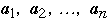
Assume we have a list of n items:

The a's are ordered by frequency of access
Probability of accessing item
 :
P(
:
P(
 )
=
)
=

Probability of looking for an item not in the list is

Average cost
-
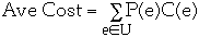
-
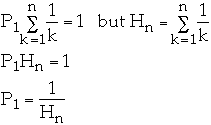
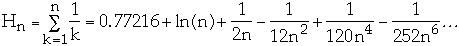
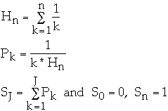
- U = set of all possible events
- P(e) = probability of event e
- C(e) = cost of event e
We have:
-
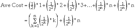
What is
 ?
?
We have:
-
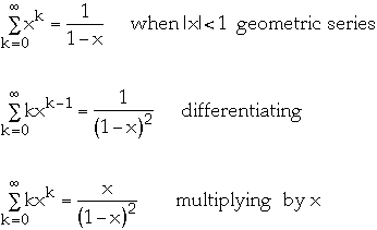
-
-
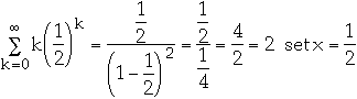
So
Thus Ave Cost =
Why linear search?
* Simple to code
	location = -1
	for (K = 0; K < n; K++)
		if ( data[K].key == X)  {
	location = K;
	break;
	}
* Requires minimal space
Organizing the list
Assume we have a list of n items:

Probability of accessing item
* Optimal Static Ordering
* Move-to-front
* Transpose
Optimal Static Ordering
Assume P(ak) is known for all k in advance
Order items in decreasing probability
Example: 2.0 average comparisons
- Let P(a) = .2
- P(b) = .4 P(c) = .3 P(d) = .1
-
- Optimal static ordering
- b, c, a, d
Move-to-front
Start with any initial ordering
When item is accessed move it to the front of the list
Example: 2.2 average comparisons
	a,	b,	c,	d	start order
	b,	a,	c,	d	accessed b	2 comparisons
	b,	a,	c,	d	accessed b	1
	a,	b,	c,	d	accessed a	2
	c,	a,	b,	d	accessed c	3
	a,	c,	b,	d	accessed a	2
	c,	a,	b,	d	accessed c	2
	c,	a,	b,	d	accessed c	1
	d,	c,	a,	b	accessed d	4
	b,	d,	c,	a	accessed b	4
	b,	d,	c,	a	accessed b	1
Transpose
Start with any initial ordering
When item is accessed move it forward one location
Example: 2.3 average comparisons
	a,	b,	c,	d	start order
	b,	a,	c,	d	accessed b	2 comparisons
	b,	a,	c,	d	accessed b	1
	a,	b,	c,	d	accessed a	2
	a,	c,	b,	d	accessed c	3
	a,	c,	b,	d	accessed a	1
	c,	a,	b,	d	accessed c	2
	c,	a,	b,	d	accessed c	1
	c,	a,	d,	b	accessed d	4
	c,	a,	b,	d	accessed b	4
	c,	b,	a,	d	accessed b	3
Permutation algorithms
- Algorithm used to rearrange list after accessing a record
Restrictions
- Only consider permutation algorithms that move accessed item forward in the
list
-
- Will not search for items not in the list
-
- All items will be searched at least once
-
- Time required by any execution of the permutation algorithm is never more
than a constant times the time required for the search immediately before that
execution.
-
- Example
- Given the list

-
- Accessing second item requires two comparisons so permutation algorithm
can take c*2 time units
-
- Accessing the last item requires two comparisons so permutation algorithm
can take c*n time units
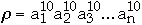
Measures of Performance
 the search sequence
 [k]
the item to be searched for on the k'th access
[k]
the item to be searched for on the k'th access
 (
( ,
k) be the state of the list after the first k accesses from [[rho]]
,
k) be the state of the list after the first k accesses from [[rho]]
 (
( ,
k)r location in the list of item r after the first k accesses from [[rho]]
,
k)r location in the list of item r after the first k accesses from [[rho]]
 =
=
 (
( ,
0) the initial configuration of the list
,
0) the initial configuration of the list
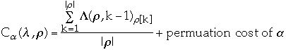
Cost of a permutation
 for a given l and r is the average cost per access in terms of the number of
probes required to find the accessed record and the work required to permute
the records afterwards
for a given l and r is the average cost per access in terms of the number of
probes required to find the accessed record and the work required to permute
the records afterwards
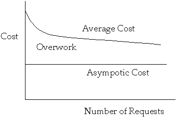
Asymptotic Cost
- Average cost over all
 and
and
 for a given

-
- Usually restrict
 to make analysis possible
Zipf noticed that in English the frequency of word usage follows:
-

where fi denotes the frequency of the ith most frequent word
Zipfian Probability Distribution:
Assume we have a list of n items:
The a's are ordered by frequency of access
Probability of accessing item
 is
is
 and
and

Then

But
 so we have
-
Zipfian Probability Distribution
Let
 for k = 1, 2, ..., n
where
Pk
n = 2

k	1	2

Pk	0.6667	0.3333


n = 3

k	1	2	3

Pk	0.5455	0.2727	0.1818


n = 4

k	1	2	3	4

Pk	0.48	0.24	0.16	0.12


n = 5

k	1	2	3	4	5

Pk	0.438	0.219	0.146	0.109	0.0876


n = 6

k	1	2	3	4	5	6

Pk	0.408	0.204	0.136	0.102	0.0816	.0680
How to Implement Zipf's Distribution
Let
-
Method 1
If
 <= rand() <
 then return k
Method 2
The number of papers in a given journal written by the same author follows an
inverse square distribution.
Let n be the total number of authors who published at least one paper in a
given journal.
The probability that a randomly chosen author contributed exactly k papers is
given by:
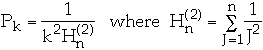
n = 2
k	1	2
Pk	0.800	0.200

n =3
k	1	2	3
Pk	0.734	0.183	0.081

n =4
k	1	2	3	4
Pk	0.702	0.175	0.078	0.043

n =5
k	1	2	3	4	5
Pk	0.683	0.170	0.075	0.042	0.027

n =6
k	1	2	3	4	5	6
Pk	0.670	0.167	0.074	0.041	0.026	0.018
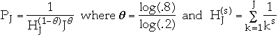
"80% of the transactions are on the most 20% of the records, and so on
recursively"
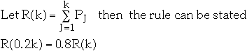
When n = 5*L we have:
-
n = 2
k	1	2
Pk	0.908	0.100

n = 3
k	1	2	3
Pk	0.858	0.100	0.063

n = 4
k	1	2	3	4
Pk	0.825	0.100	0.063	0.047

n = 5
k	1	2	3	4	5
Pk	0.800	0.100	0.063	0.047	0.038
80% - 20% Rule
Knuth claims we can approximate this by:
n = 2
k	1	2
Pk	0.644	0.355

n = 3
k	1	2	3
Pk	0.515	0.283	0.200

n = 4
k	1	2	3	4
Pk	0.446	0.245	0.173	0.135

n = 5
k	1	2	3	4	5
Pk	0.401	0.220	0.155	0.121	0.100

n = 6
k	1	2	3	4	5	6
Pk	0.369	0.203	0.143	0.111	0.092	0.078
Steady State
- Further permutations are not expected to change the expected search time
significantly
-
Locality
- Subsequences of [[rho]] may have relative frequencies of access that are
drastically different from the overall relative frequencies
-
-

-
Total Number of Comparisons in searchWorst Case
	n	Move-to-Front	BST
	7	112	170
	15	360	490
	31	1240	1290
	63	4536	3210
Measures of Convergence
Relative Measurements
- Optimal Static Ordering - items are ordered by static probability of access
and are not moved
-
-
-
Total Number of Comparisons in searchWorst Case
	n	Move-to-Front	OSO
	7	112	210
	15	360	1050
	31	1240	4650
Move-to-front
-
- Assume Zipf distribution
-
-
-
-

-
-
Transpose
-
Count
- approaches optimal static ordering
Comparisons between Algorithms
No Optimal Memoryless algorithm
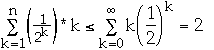
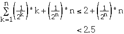
Asymptotic Cost
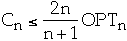
- Move-to-front asymptotic cost at most twice asymptotic cost of the optimal
static ordering
-
- Asymptotic cost of transpose is <= asymptotic cost of move-to-front
-
- Count is asymptotically equal to optimal static ordering
-
Worst Case
- Move-to-front and count at most twice the worst case of the optimal static
ordering
-
- Transpose can be far worse
-
- Moving a record any fraction of the distance to the front of the list will
be no more than a constant times the optimal off-line algorithm
-
- The constant is inversely proportional to the fraction of the total
distance moved